What is a curve.
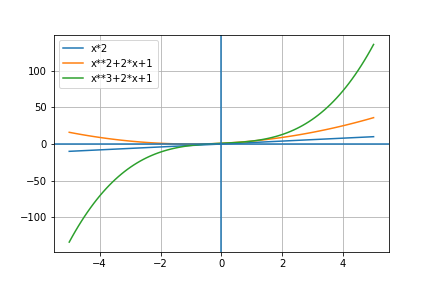
A curve is a path inscribed into a dimensional space. We are all familiar with curves in euclidian space such as 2 dimensional space where polynomial functions describe a path through that 2-d space. We see below some well know polynomial functions graphed in a small range.

in these examples, the single x value is mapped onto the output y value for the range[-5,5] of x.
Space filling curve
A space filling curve is a parameterized function which maps a unit line segment to a continuous curve in the unit space (square, cube, ….). For the unit square form we have i in range[0..1] with a function F(i) that provides output x,y with 0<=x,y,<=1.
The Hilbert Curve
The Hilbert curve is a curve which uses recursion in its definition and it is a continuous fractal so as its order increases it gets more dense but maintains the basic properties of the curve and the space that the curve fills.

In the space in which this curve is inscribed (x,y) where 0<=x,y,<=1 we can see that as the order (complexity) of the curve increases, it does a better job of filling in the space. Another way to consider this is that the x and y input for low order are like low resolution numbers along the lines of the resolution of an Analog to Digital (A/D) convertor.
A 1 bit A/D convertor can only indicate the presence or absence of a signal while a 12bit A/D convertor can capture significant signal resolution.
The lowest order Hilbert curve starts with x and y values being either 0 or 1 which gives us the simple “U” pattern which have x,y coordinates of [(x=0,y=1),(0,0),(1,0),(1,1)]
At each point along the curve it also has a value in the range [0,1], so again the simple example, would have the function map
(0,1) -> 0, (0,0)->0.33, (1,0)-> 0.66 and (1,1)->1
As the x,y resolution of the curve increases then its possible for number of curve values to become larger to the point where is we leave the A/D convertor example where x and y become real numbers then the curve values can also be a real number between 0 and 1.
If we say that our input parameters are (x,y) and curve output value is z at point (x,y) then the hilbert curve has an interesting and very attractive property that values of x and y representing points that are close to each other will generate values of z that are also close to each other. This property allows for (in our example) 2 dimensional closeness to be mapped onto numbers that retain the ability to measure closeness but using only 1 dimension.
So far I have been using a 2 dimensional example where the space filling curve traverses a 2 dimensional space, but its also possible to have a 3 dimensional curve that traverse a 3 dimensional space and also in higher dimensions. This effectively provides a method for high dimensional data to be mapped onto a simple dimensional value where some inherent properties of the high dimension data are maintained in the linear representation.
In the video above of a 3 dimension hibert curve, you can see that 3d spacial distance maps onto closeness of the value of the curve.
Once we have a space filling curve with points [0<=x<=1,0<=y<=1] that mops to values h range(0 ->1) then we can use this to have easy calculations for relative closeness which are simple calculations (number subtraction) instead of euclidian distances calculations that involve squaring and square root calculations. This may not seem like a big deal in 2 dimensions but as the number of dimensions grows having an simple calculation to derive closeness will be an interesting capability.
Future plans
In later posts, I want to use this capability to have items that are arranged in a number of different spaces and using hibert spaces to allow for easy inference of closeness within these spaces. One example of this is the fact that ip addresses are not geographically allocated so having a method that allows ip addresses to be attached to positions in a hilbert space will provide an easy scalable method of understanding the geographic proximity of ip addresses – for instance, a computation to decide what ip addresses are close to a city or an address will involve taking the gps coordinates of the city, transforming them in the hilbert number and then a definition of closeness will be a range [h-∂, h+∂] which can be then traversed to find all the ip addressed within that space.
