
Continuing the theme (part1, part2) of using GPS data to augment network graph data, this post will consider using the data for inclusion in the network graph but will also introduce taking the network graph and rendering this onto a geographical mapping visualization.
NetworkX graph package
In these discussions I have been using the Python NetworkX package to store a graph structure, nodes in this graph have city names as identifiers and edges created as a tuple or pair of city names.
import networkx as nx
import matplotlib.pyplot as plt
G = nx.Graph()

Cnames = ['Vancouver', 'Portland', 'San Francisco', 'Seattle',
          'San Antonio', 'Dallas', 'Austin', 'Sevilla',
          'Belfast', 'Sydney', 'Canberra', 'Tokyo']
G.add_node(name)
G.add_edge(name,'Dublin')
The NetworkX package allows for easy graph creation and manipulation, allows attributes to be added to the graph structure and then the package graph algorithms ( shortest path, cliquing, graph analysis) and also graph traversal, neighbor query and also graph drawing using standard plotting packages such as matplotlib.
plt.figure(figsize=(8, 8))
pos = nx.spring_layout(G)
nx.draw(G,nodelist=nodes,with_labels=True,pos=pos)
_ = nx.draw_networkx_edge_labels(G,pos=pos)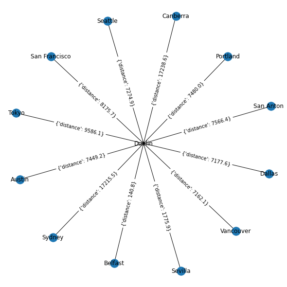
Graph attributes, added and calculated
At this point, we now have a capability to generate a network graph that has named nodes and edges. The edges of the graph have a calculated distance derived from the GPS location of the nodes. An application of interest to me is calculating a idealized latency value for the network, i.e. what is the idealized one-way latency between location x and location y.
One-way latency for model
For the global network model that we have incrementally built, we started with cities as nodes of the network, using the GPS coordinates of these cites we create graph edges between the cities and calculated the great circle distance between these cities.
The next step in this model is to assume that a single fiber optic runs between these cities. This is unrealistic for geographical, technical, electro/optical and political reasons but is adequate for the model that I am building.
Light traveling in a fiber optic travels at a different speed than in free space. In free space light travels at 299792458 m/s (approximated as 3×10^5m/s). In an optical fiber, light travels slower than in free space, approximately 35% slower based on the refractive index of the fiber optic between its core and its cladding.
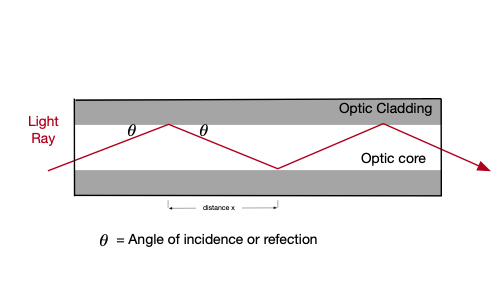
A fiber optic is composed of two different materials, the optic core and the optic cladding. As light leaves the optic core and enters the optic cladding it is refracted, at a certain angle (called the critical angle) the refraction results in the light being totally reflected back into the optic core. This results as shown in the figure above have the light ray ‘bouncing’ along the fiber optic from one end to another.
In the figure an angle θ is shown as the incident and relected angle, there is also a distance X marked which shows the linear distance along the fiber from one reflection point to another. While the light would traveling horizontally the distance of x when its in free space, because the light is inside the fiber optic it has to travel a longer distance donated as x/sin(θ), so lets assume θ = 45 degrees, sin(45 deg) = 0.707 so the light in the fiber optic has to travel x/0.707 which in this example is 1.41 times x, thus the earlier rule of thumb of light traveling 35% slower in an fiber optic.
So this 35% figure we can say a modeled speed of light is 2.121X10^5 m/s can be used.
nodes = []
for name in Cnames:
    nodes.append(name)
    G.add_node(name)
    G.add_edge(name,'Dublin')
    distance  = great_circle(Cities['Dublin'],
                             Cities[name]).kilometers
    G.edges['Dublin',name]['distance'] = round(distance,1)
    G.edges['Dublin',name]['oneway-latency'] =
                         distance * 2.121*10^^5
This latency calculation is assuming that the fiber optic is laid in a ‘straight line’ along the great circle between the two locations and does not include any optical regenerators, or intervening optical, or networking equipment.