
In a previous post, I introduced the concept of space filling curves and the ability to take a high dimension space and reduce it to a low or 1 dimension space. I also showed the complexity in 2 dimensions and in 3 dimensions of the Hilbert Curve which I hope also provided an appreciation for the ability of the curve to traverse the higher dimension space.
In practice there are a number of implementations of the Hilbert curve mapping available in a number of languages including:
- https://github.com/tammoippen/geohash-hilbert
- https://github.com/google/hilbert
- https://github.com/galtay/hilbertcurve
From galtay we have the following example where the simplest 1st order 2 dimension hilbert curve maps 4 integers [1,2,3,4] onto the 2 dimensional space <x,y> x = (0|1), y = (0|1)
>>> from hilbertcurve.hilbertcurve import HilbertCurve
>>> p=1; n=2
>>> hilbert_curve = HilbertCurve(p, n)
>>> distances = list(range(4))
>>> points = hilbert_curve.points_from_distances(distances)
>>> for point, dist in zip(points, distances):
>>>     print(f'point(h={dist}) = {point}')

point(h=0) = [0, 0]
point(h=1) = [0, 1]
point(h=2) = [1, 1]
point(h=3) = [1, 0]
its also possible to query the reverse transformation going from a point in the space to a distance along the curve.
>>> points = [[0,0], [0,1], [1,1], [1,0]]
>>> distances = hilbert_curve.distances_from_points(points)
>>> for point, dist in zip(points, distances):
>>>     print(f'distance(x={point}) = {dist}')

distance(x=[0, 0]) = 0
distance(x=[0, 1]) = 1
distance(x=[1, 1]) = 2
distance(x=[1, 0]) = 3
On galtay’s repositary, there is a graphic that shows 1st order, 2nd order and 3rd order curves in an <x,y> space. The ranges represented by each of the curve get more resolution as the order increases:
- 1st order curve supports values (0|1) on the x and y axis giving us a 2 bit binary number of range values i.e. 00, 01, 10,11 -> 0..3
- the 2nd order curve is more complex and (0|1|2|3) on the x and y axis giving us a 4 bit number of range values, 0000, 0001 0010….1111 -> 0..15
- the 3rd curve includes the x,y values to 6 bits of resultion giving values 0->63.
As I have noted, an increase in the order of the curve, increases it complexity ( wiggleness) and its space covering measure and also provides more range quanta along the curve.
Returning to my suggestion in the earlier post, that the curve can be used to map a geographic space into the range and then have a entity (ip addresses which by themselves have no geographic relationship mapped not onto the range. in this fashion, subtraction along the range provides a (resolution dependant) measure of closeness of the location of these ip addresses.
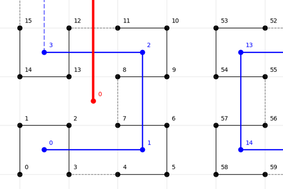
Using galtay rendering of the 3 order curve shown in back, if one focuses on the value 8 along the curve, its specially close in 2 dimensions 13,12,11,10,9,7,6,2 but not specially close to 63 or 42 which are rendered outside the area shown. With simple subtraction we see can have rule that says ip addresses within 5/6 units the 8 are close to whereas ip addresses with 20, 30,40 units distance are further away. As the order of the curve increases, this measurement get a better resolution.