Exploring space filling curves.

What is a curve.

A curve is a path inscribed into a dimensional space. We are all familiar with curves in euclidian space such as 2 dimensional space where polynomial functions describe a path through that 2-d space. We see below some well know polynomial functions graphed in a small range.

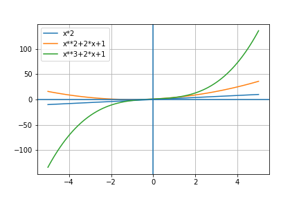
in these examples, the single x value is mapped onto the output y value for the range[-5,5] of x.

Space filling curve

A space filling curve is a parameterized function which maps a unit line segment to a continuous curve in the unit space (square, cube, ….). For the unit square form we have i in range[0..1] with a function F(i) that provides output x,y with 0<=x,y,<=1.

The Hilbert Curve

The Hilbert curve is a curve which uses recursion in its definition and it is a continuous fractal so as its order increases it gets more dense but maintains the basic properties of the curve and the space that the curve fills.

Hilbert Curve: TimSauder, CC BY-SA 4.0

In the space in which this curve is inscribed (x,y) where 0<=x,y,<=1 we can see that as the order (complexity) of the curve increases, it does a better job of filling in the space. Another way to consider this is that the x and y input for low order are like low resolution numbers along the lines of the resolution of an Analog to Digital (A/D) convertor.

A 1 bit A/D convertor can only indicate the presence or absence of a signal while a 12bit A/D convertor can capture significant signal resolution.

The lowest order Hilbert curve starts with x and y values being either 0 or 1 which gives us the simple “U” pattern which have x,y coordinates of [(x=0,y=1),(0,0),(1,0),(1,1)]

At each point along the curve it also has a value in the range [0,1], so again the simple example, would have the function map

(0,1) -> 0, (0,0)->0.33, (1,0)-> 0.66 and (1,1)->1

As the x,y resolution of the curve increases then its possible for number of curve values to become larger to the point where is we leave the A/D convertor example where x and y become real numbers then the curve values can also be a real number between 0 and 1.

If we say that our input parameters are (x,y) and curve output value is z at point (x,y) then the hilbert curve has an interesting and very attractive property that values of x and y representing points that are close to each other will generate values of z that are also close to each other. This property allows for (in our example) 2 dimensional closeness to be mapped onto numbers that retain the ability to measure closeness but using only 1 dimension.

So far I have been using a 2 dimensional example where the space filling curve traverses a 2 dimensional space, but its also possible to have a 3 dimensional curve that traverse a 3 dimensional space and also in higher dimensions. This effectively provides a method for high dimensional data to be mapped onto a simple dimensional value where some inherent properties of the high dimension data are maintained in the linear representation.

In the video above of a 3 dimension hibert curve, you can see that 3d spacial distance maps onto closeness of the value of the curve.

Once we have a space filling curve with points [0<=x<=1,0<=y<=1] that mops to values h range(0 ->1) then we can use this to have easy calculations for relative closeness which are simple calculations (number subtraction) instead of euclidian distances calculations that involve squaring and square root calculations. This may not seem like a big deal in 2 dimensions but as the number of dimensions grows having an simple calculation to derive closeness will be an interesting capability.

Future plans

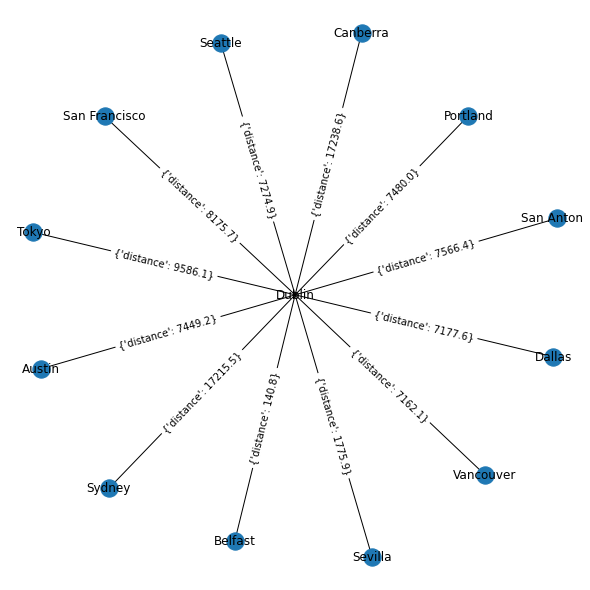
In later posts, I want to use this capability to have items that are arranged in a number of different spaces and using hibert spaces to allow for easy inference of closeness within these spaces. One example of this is the fact that ip addresses are not geographically allocated so having a method that allows ip addresses to be attached to positions in a hilbert space will provide an easy scalable method of understanding the geographic proximity of ip addresses – for instance, a computation to decide what ip addresses are close to a city or an address will involve taking the gps coordinates of the city, transforming them in the hilbert number and then a definition of closeness will be a range [h-∂, h+∂] which can be then traversed to find all the ip addressed within that space.

Tesla Solar Roof Install

While out walking this afternoon I came across an ongoing Tesla Solar Roof in the neighborhood. Last week, the old roof had been taken off the house and an under covering which was branded Tesla had been installed so I kinda guessed that the Tesla Solar roofing was the next step.

True to fashion, a large work party, with truck and a sign advertising that it was a Tesla install appeared this AM. This afternoon I checked on their progress and the the panel installs have begun.

The individual tiles seemed to be delivered in palleted boxes and one is show below.

The picture I believe is showing 4 panels with the black triangular piece being the attachment point to the roof. I will have to investigate more it seems like the panels have significant space underneath them and they must be sturdy as the installer seem to be walking on them (with soft shoes) in the above picture.

Once the dust has settled I will speak with the homeowner to get some more information on the size of the install. I did a quick search and entering the Telsa Solar roof site and getting a price/recommendation it the following were some recommendations.

Size Roof cost power walls price after incentives etc
4.1KW $31166 1 for 7770 $36,748, $31166 after incentive
10.2KW $36867 3 for $17390 $45,552, $38867 after incentive
Pricing for two sizing of roof from Tesla site.

All in all, its looks like a pretty expensive setup, where there is marginal price difference between the 4.1KW panel setup and 10.2KW setup. Checking on Amazon, Renogy 30pcs 320W Monocrystalline Solar Panels would set you back $9700 which is close enough to 10KW of panels, so yes there is a lot of wiring, framing, installation and permitting costs but is it $20K? But its Tesla so it must be good for you…… I assume that Tesla will get the unit costs of the solar panels down with mass adoption.

Adding calculated distance to network maps calculated from GPS coordinates.

Continuing the theme (part1, part2) of using GPS data to augment network graph data, this post will consider using the data for inclusion in the network graph but will also introduce taking the network graph and rendering this onto a geographical mapping visualization.

NetworkX graph package

In these discussions I have been using the Python NetworkX package to store a graph structure, nodes in this graph have city names as identifiers and edges created as a tuple or pair of city names.

import networkx as nx
import matplotlib.pyplot as plt
G = nx.Graph()

Cnames = ['Vancouver', 'Portland', 'San Francisco', 'Seattle', 
          'San Antonio', 'Dallas', 'Austin', 'Sevilla', 
          'Belfast', 'Sydney', 'Canberra', 'Tokyo']
G.add_node(name)
G.add_edge(name,'Dublin')

The NetworkX package allows for easy graph creation and manipulation, allows attributes to be added to the graph structure and then the package graph algorithms ( shortest path, cliquing, graph analysis) and also graph traversal, neighbor query and also graph drawing using standard plotting packages such as matplotlib.

plt.figure(figsize=(8, 8))
pos = nx.spring_layout(G)
nx.draw(G,nodelist=nodes,with_labels=True,pos=pos)
_ = nx.draw_networkx_edge_labels(G,pos=pos)

Graph attributes, added and calculated

At this point, we now have a capability to generate a network graph that has named nodes and edges. The edges of the graph have a calculated distance derived from the GPS location of the nodes. An application of interest to me is calculating a idealized latency value for the network, i.e. what is the idealized one-way latency between location x and location y.

One-way latency for model

For the global network model that we have incrementally built, we started with cities as nodes of the network, using the GPS coordinates of these cites we create graph edges between the cities and calculated the great circle distance between these cities.

The next step in this model is to assume that a single fiber optic runs between these cities. This is unrealistic for geographical, technical, electro/optical and political reasons but is adequate for the model that I am building.

Light traveling in a fiber optic travels at a different speed than in free space. In free space light travels at 299792458 m/s (approximated as 3×10^5m/s). In an optical fiber, light travels slower than in free space, approximately 35% slower based on the refractive index of the fiber optic between its core and its cladding.

A fiber optic is composed of two different materials, the optic core and the optic cladding. As light leaves the optic core and enters the optic cladding it is refracted, at a certain angle (called the critical angle) the refraction results in the light being totally reflected back into the optic core. This results as shown in the figure above have the light ray ‘bouncing’ along the fiber optic from one end to another.

In the figure an angle θ is shown as the incident and relected angle, there is also a distance X marked which shows the linear distance along the fiber from one reflection point to another. While the light would traveling horizontally the distance of x when its in free space, because the light is inside the fiber optic it has to travel a longer distance donated as x/sin(θ), so lets assume θ = 45 degrees, sin(45 deg) = 0.707 so the light in the fiber optic has to travel x/0.707 which in this example is 1.41 times x, thus the earlier rule of thumb of light traveling 35% slower in an fiber optic.

So this 35% figure we can say a modeled speed of light is 2.121X10^5 m/s can be used.

nodes = []
for name in Cnames:
    nodes.append(name)
    G.add_node(name)
    G.add_edge(name,'Dublin')
    distance  = great_circle(Cities['Dublin'],
                             Cities[name]).kilometers
    G.edges['Dublin',name]['distance'] = round(distance,1)
    G.edges['Dublin',name]['oneway-latency'] = 
                         distance * 2.121*10^^5

This latency calculation is assuming that the fiber optic is laid in a ‘straight line’ along the great circle between the two locations and does not include any optical regenerators, or intervening optical, or networking equipment.

Calculating the distance between 2 GPS Cordinates – Follow on

In a previous post, I discussed calculating distances based on GPS coordinates, subsequently I came across a good python library that offers this functionality as well as a lot more. I decided that anybody that is interested in the distance calculation via GPS coordinates will probably appreciate everything else that the GeoPy library has to offer.

In addition to the distance calculation, GeoPy offers a client functionality to access several popular geocoding web servers.

From the Readme file of the package’s GitHub site:

geopy makes it easy for Python developers to locate the coordinates of addresses, cities, countries, and landmarks across the globe using third-party geocoders and other data sources.

geopy includes geocoder classes for the OpenStreetMap NominatimGoogle Geocoding API (V3), and many other geocoding services.

Here is my previous example coded with the GeoPY library

from geopy.distance import great_circle
Dublin = (53.35, -6.27)
SanFrancisco=(37.78, -122.42)

great_cicle_dis = great_circle(Dublin, San Francisco).kilometers
geodesic_dis = geodesic(Dublin, San Francisco).kilometers

Cities = { 'Vancouver':(49.25,-123.1),
    'Portland':(45.52,-122.68),
    'San Francisco':(37.78, -122.42),
    'Seattle':(47.62, -122.33),
    'San Antonio':(29.42, -98.5),
    'Dallas':(32.78,-96.8),
    'Austin':(30.25,-97.75),
    'Dublin':(53.35, -6.27),
    'Sevilla':(37.38, -5.98),
    'Belfast':(54.6,-5.93),
    'Sydney':(-33.87, 151.22),
    'Canberra':(-35.3, 149.12),
    'Tokyo':(35.68, 139.7)}

import networkx as nx
import matplotlib.pyplot as plt
G = nx.Graph()
Cnames = ['Vancouver', 'Portland', 'San Francisco', 'Seattle', 
          'San Antonio', 'Dallas', 'Austin', 'Sevilla', 
          'Belfast', 'Sydney', 'Canberra', 'Tokyo']
nodes = []
for name in Cnames:
    nodes.append(name)
    G.add_node(name)
    G.add_edge(name,'Dublin')
    distance = great_circle(Cities['Dublin'],Cities[name]).kilometers
    G.edges['Dublin',name]['distance'] = round(distance,1)
plt.figure(figsize=(8, 8))
pos = nx.spring_layout(G)
nx.draw(G,nodelist=nodes,with_labels=True,pos=pos)
_ = nx.draw_networkx_edge_labels(G,pos=pos)

A complete example is provided in the following GitHub page

The GeoPy library is well worth reviewing as it also have a litany of functions which I did not cover here including:

Geocoding is provided by a number of different services, which are not affiliated with geopy. These services provide APIs, which anyone could implement, and geopy is a library which provides these implementations for many different services in a single package.

Calculating the distance between 2 GPS points

With the proliferation of GPS tagging in data sets, a useful calculation to that allows to derive the distance between two points is possible using the Haversine formula. The law of havershines is a more general formula within spherical trigonometry which relates to sides and angles or spherical triangles. On the surface of a sphere the ‘straight line’ connecting two points is actually the arc of a curve on the sphere surface. This curve arc is a arc along a great circle on the sphere and is mathematically called the spherical distance.

In the haversine calculation, the radius of the earth varies around 6356.752 km to 6378.137 km so choosing a value will result in a error that can not be less than 0.5%.

From wikipedia, the calculation is defined as:

so using this formula, the distance of the great circle arc between two points on earths surface in python is:

from math import asin, cos, radians, sin, sqrt
def arclen(lat_a,lon_a,lat_b,lon_b):
  r = 6370 #note this is for KM distance
  a1,a2, = (radians(lat_a),radians(lon_a)) 
  b1,b2 = (radians(lat_b),radians(lon_b))
  delta_lat = b1-a1
  delta_lon = b2-a2
  n = abs(sin(delta_lat/2) **2 
          + cos(a1)*cos(a2)*(sin(delta_lon/2) **2))
  if n >1:
    n = 1
  return 2*r*asin(sqrt(n))

A Jupiter notebook with an more extensive example is available.